CLV
As you may know (or not, in which case please read this article), CLV is one of the most important metrics for your store. Not only does it help you know your store’s actual value, but it is also key as to how much money you can spend in acquiring customers, for it tells you how much money they’re gonna ‘give you back’.
Ironically, though, CLV is one of the most under-estimated and overlooked metrics. Many startups don’t even calculate it, and many who do only sum all the revenue they’ve ever had and divide it equally between all users.
This approach however not only is pretty basic, but it deliberately lets out a key piece of truth: not all customers are equal. You’ll have people who buy $1,000 from you, but you’ll also have customers who only came in attracted by a massive discount, and won’t buy again unless they again see an insane price drop.
Does it really matter? Absolutely.
First of all, bad customers can be very bad business: by giving huge discounts, and adding all the marketing and operations costs, you can easily be left without profit, or even lose money acquiring those cheap customers.
So, you’ll want to identify the kind of customers who will bring you more money in the long run, and bring more of them, as many as you can. As for the low quality customers… You’ll want to bring as few of them as you can.
However, to do this, you can’t be just looking backwards and seeing how much people end up spending on your site when there’s nothing more to do. To actually take action, you’ll need to know both how much a customer has spent and how much he will spend in the future.
Sounds impossible, doesn’t it? It’s not. We created a tool that tells you exactly how much revenue each one of your customers will bring you in the future, and when they will do it. So you can pamper those good customers, create stronger bonds with them and upsell… And stop worrying and losing money over the bad customers.
The outcome
You can expect 2 very different things from our model:
1) Forward-looking (predicted) values
We predict for you:
- your customers’ average CLV (how much money an average customer will bring to you during their lifetime)
- every customer’s LTV.
- a lists of the top places for you. We’ll tell you exactly how much money you will receive from each demographic location (cities, states and countries)
- list of top 1st products/categories. We’ll find the customers who are expected to spend more money during their entire lifetime. We’ll then find which was the first product they ever bought with you, and which category that product belongs to. This is really big in identifying potential good customers: we’re finding relations between lifetime spend and the first product purchased, so you’ll be able to tell with some degree of certainty, from the very first order someone places with you, if they will be good or bad customers.
2) Backward-looking (historical) data.
All of the above are things we’ll predict from the future… But we’ll also give you insights on what has already happened in your store:
- Monthly new vs old customers
- The places where you’ve sold the most (by country, city and state)
- The products and categories you’ve sold the most.
- Insights on which places, products and categories are rising (selling more than before) and which are falling (selling less than before)
The actual model
As it does involve quite some math, we’ll explain this in 2 leves of complexity, so if you don’t really want to know exactly all the details of our calculations, you can read only the basic explanation and you’re good to go.
a) Basic
The short version is we do mathematical modeling with your data. Modeling (in math) means watching the past behavior and using it to predict the future behavior of a person or group of people. That’s what we do: we take your past data, feed it to a model, and out come the predictions. We use 2 models: the first one to know when people are going to buy, and another one to know how much money they will spend in each of those orders. The models we use are like superstar for calculating CLV: they were developed by mathematicians and backed up by more than 20 years of research, so you can be assured they work damn well.
b) Advanced
If you want to know a little bit more, we’ll tell you not all modeling is good. If you do it wrong, you can end up with predictions that have nothing to do with reality. For example: if your predictions are way lower than the actual facts, you’ll end up with a massive shortage of inventory, which means you’ll ‘lose’ the money you could had made by selling those units. This is called opportunity cost. If on the contrary you predict sky rocketing sales, you’ll both have lots of inventory that won’t get sold, and most likely also spend lots of money in advertising, so you’ll actually be losing money on two fronts.
Worried? Don’t be. As we said before, the models we use were developed and perfected by PhD mathematicians form universities like MIT, and are featured in many scientific publications in respected science magazines like Elsevier. In this section we’ll explain the first model, called Beta-Geometric model (for short BG). This is the one used to know when and how many times people will place an order. The second model we used is called Gamma-Gamma, but we won’t go over it in this section.
Every single model makes assumptions about the data. These are the cornerstones for defining the whole model. Depending on how accurate (or not) these assumptions are, things can go really well (or not).Our assumptions involve probability distributions. This is where things start to get a bit technical, so if you think you’ve read enough, just skip to the next section.
Before we move on, we want to state a simple but crucial fact for all CLV calculations: not all customers in your database are worth the same, and not all of them are active. There are many who have already bought what they needed, and won’t ever buy again. And it’s ok. It’s only natural. What you want to do, however, is a) stretch the time during which they’ll come and buy (their lifetime), and b) make them buy as much as you can during that period (their lifetime value, or CLV). That’s the notation we’ll use: active are the customers who will still make another purchase with you. Churned, lost or inactive customers are the ones who won’t ever buy again.
Ok, so, moving on. These are 5 key assumptions we make:
- Customer activity. We assume that, for every customer in your store the behavior is: first the buy a little. Then they see your product is good, or see your store is not a scam, or they’ve already seen your catalogue looking for the initial item and found another one they liked, so they’ll buy more. It’s only natural, they first try it, and when they know it, or even know of it, they get confident and spend more. After giving you lots money, though, their activity starts declining, until they eventually stop buying from you. This behavior is seen in every single e-commerce. You may think yours is different… It’s not. What IS different is how fast customers will go from spending a little to spending big to going back to spending little. Another thing that does change is how big those leaps are: how much more they spend when they spend more, and how much less they spend when they spend less.
All of this is modeled by what is called ‘Poisson distribution’. Basically, what we say is that for every customer, his purchases will be in the shape of a curve like the one of the following:
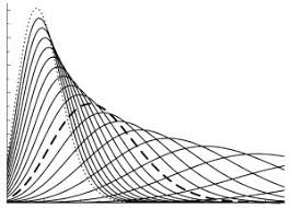
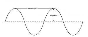
Which curve, though, that will depend both from that particular customer, and from your business model. Poisson distribution has 2 parameters, λ and k, which determine what we could call the ‘amplitude’ and ‘wavelength’ of the curve.
Here, λ is the transaction rate of your customers, ie, how many times they buy in a given period of time. When you model something using a probabilistic distribution, what you do is called ‘fitting the parameters’ λ and k, to find the pair that best adapts to every customer.
- Transaction rate similarity. We assume every single customer behaves differently. He/she is unique and so are their habits. However, there is some pattern of behavior: you’ll probably have seen that you have many customers who don’t buy much, and a small chunk of customers who spend lots and lots of money with you. This heterogeneity also follows a probability distribution, the Gamma distribution.
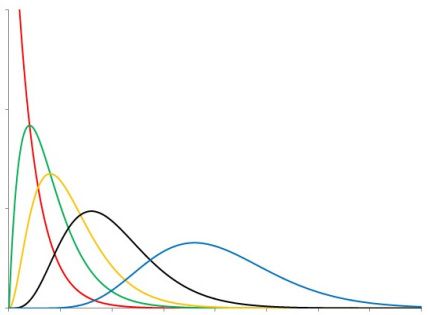
This curve is similar to the Poisson one. This distribution also has two parameters, and it will model how the λfrom the Poisson distribution varies across customers. A way to understand this is that the horizontal axis is how many times they buy from you (eg: 5 purchases), and the vertical one how many customers fall into that category (how many of your customers place 5 orders during their lifetime).
- Inactivity. We assume the inactivity of a customer comes right after the last transaction they made. If someone bought from you son May 1st and never came back, we’ll say he became inactive May 1st after his purchase. Now, how can we know in advance when a customers’ last purchase will be? Once again, we use probability, and once again a probabilistic distribution enters the scene. Now it’s a geometric distribution:
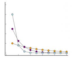
The geometric distribution is a special case of the Poisson. Here what we basically assume is that after the first transaction, probability of churning (or never returning) is much higher tan after a couple (or a lot of) purchases. The probability is always greater than 0, but is much smaller as time goes by. Again, this is a fair assumption for the more a customer buys with you, the more loyal he becomes to the brand. After all, there’s a reason why (s)he keeps coming back, right?
- Inactivity similarity. Again, even assuming every customer is different, because of your business model there will be some similarities between you customers. For example, if you sell mattresses, you’ll expect customers to come back and buy much less than you would if you were a food delivery service. Mathematically, this means that the probability of churning also follows a probabilistic distribution. This time, it’s a beta distribution
- Customer uniqueness. Every customer is absolutely unique. If Mary suddenly decides she doesn’t want any business with you, that does not affect Bob’s purchases. Likewise, if you convince Tony that your brand is absolutely fantastic and get him to spend lots of money, that won’t affect John’s purchasing behavior. So, the transaction rates and the probabilities of churning vary independently between customers
If you want to know more about what you can do with your CLV and how to make the most of it, read this article. If you have any more doubts either regarding the models, what you can do with them, or any other subject for that matter, please feel free to contact us!